Quantitative Techniques — 2024
KNEC Diploma in Supply Chain Management, Module II. Original theory examination questions with explained model answers for revision.
November 2024
Paper codes: 2903/204
Time: 3 hours
Instructions: Answer any FIVE questions. All questions carry equal marks. Answer the questions in English.
Question 1(a) — 10 marks
The following are the average revenue (AR) and average cost (AC) functions of a product manufactured and sold by Baraka Limited.
AR = 40 − 0.5q
AC = 15 + 2qWhere q is the quantity produced and sold.
(i) Derive the profit function.
(ii) Determine the: I. quantity that maximizes profit; II. maximum profit.
Model answer
| Step | Working |
|---|---|
| Total revenue | TR = q × AR = 40q − 0.5q² |
| Total cost | TC = q × AC = 15q + 2q² |
| Profit function | π(q) = TR − TC = 25q − 2.5q² |
| First-order condition | dπ/dq = 25 − 5q = 0 ⇒ q = 5 units |
| Maximum check | d²π/dq² = −5 < 0 |
| Maximum profit | π(5) = 25(5) − 2.5(25) = 62.50 monetary units |
Question 1(b) — 10 marks
Given the following matrices:
A =
3 2 4 -1 6 0 B =
4 1 3 2 C =
4 5 Determine: (i) Aᵀ; (ii) B⁻¹; (iii) B × C; (iv) Cᵀ × B.
Model answer
(i) Transpose A by swapping rows and columns: Aᵀ =
| 3 | 4 | 6 |
| 2 | -1 | 0 |
(ii) det B = 4×2 − 1×3 = 5. Swap diagonal entries and change the signs of off-diagonal entries, then divide by 5: B⁻¹ = (1/5)
| 2 | -1 |
| -3 | 4 |
(iii) BC: first row 4×4 + 1×5 = 21; second row 3×4 + 2×5 = 22.
| 21 |
| 22 |
(iv) CᵀB: [4,5]B = [4×4 + 5×3, 4×1 + 5×2] =
| 31 | 14 |
Question 2(a) — 10 marks
Explain five limitations of quantitative techniques in business decision making.
Model answer
- Results depend on reliable data; incomplete, biased or outdated figures can produce misleading recommendations.
- Models simplify reality and depend on assumptions that may not hold in changing business conditions.
- Qualitative factors such as morale, ethics and customer relationships are difficult to express fully as numbers.
- Building and maintaining models may require costly data systems, specialist staff and time.
- Managers may misinterpret precise-looking results or apply them beyond the model’s scope; judgement and sensitivity checks remain necessary.
Question 2(b) — 10 marks
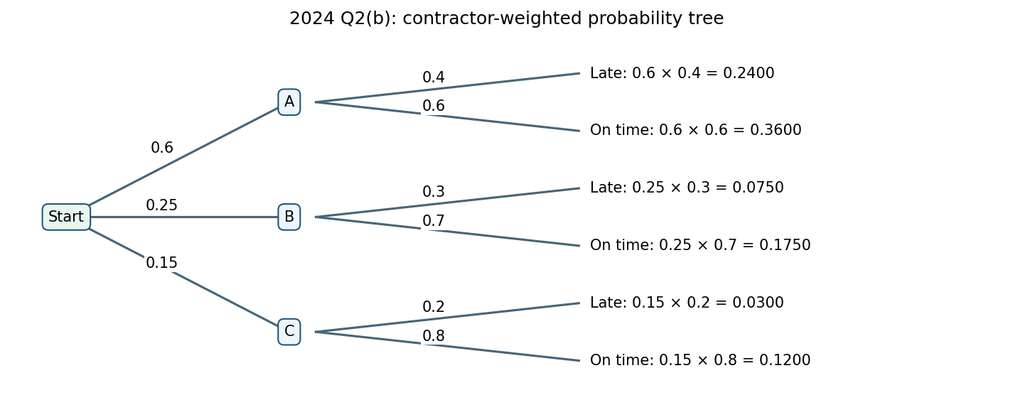
Odok Limited hired three contractors A, B and C to construct a road. The contractors have been assigned 60%, 25% and 15% of the road respectively. The probabilities that contractors A, B and C will fail to complete the construction within the scheduled time is 0.4, 0.3 and 0.2 respectively.
(i) Present the information above using a tree diagram.
(ii) Determine the probability that the road construction will: I. not be completed as scheduled; II. be completed as scheduled.
Model answer
The usual weighted-tree interpretation selects a road section at random, with contractor probabilities equal to the assigned proportions. Multiply probabilities along each branch, then add mutually exclusive paths.
| Step / item | Working | Result |
|---|---|---|
| Not completed on time | 0.60×0.40 + 0.25×0.30 + 0.15×0.20 | 0.34 |
| Completed on time | 0.60×0.60 + 0.25×0.70 + 0.15×0.80 | 0.66 |
Interpretation: these are the probabilities for a randomly selected section (or expected proportions of road), as implied by the supplied weights. If “the road” literally means every contractor finishing on time, the weighted sum is not that event. Under an additional independence assumption, P(all finish) = 0.6×0.7×0.8 = 0.336 and P(at least one late) = 0.664. Independence is not stated, so the whole-road probability is otherwise undetermined.
Question 3(a) — 8 marks
Outline the steps that are followed in the test of hypothesis.
Model answer
- State the null hypothesis H₀ and the alternative hypothesis H₁ in terms of the population parameter.
- Choose the significance level α before inspecting the result.
- Select a suitable test and verify its assumptions and the sampling design.
- Specify whether the test is one-sided or two-sided from the alternative hypothesis.
- Identify the sampling distribution and the critical region, or plan to use a p-value.
- Calculate the test statistic from the sample data.
- Reject H₀ if the statistic enters the critical region or p ≤ α; otherwise fail to reject H₀.
- Interpret the conclusion in the business context, stating what the evidence supports without claiming that failure to reject proves H₀ true.
Question 3(b) — 12 marks
A survey conducted in a certain country in Kenya found that 55% of the families own mobile phones. Ten families were randomly selected from the county. Determine the probability that:
(i) none of the 10 families have mobile phones;
(ii) at least one of the 10 families have mobile phones;
(iii) all the 10 families have mobile phones;
(iv) fewer than 4 families have mobile phones;
(v) more than 8 families do not have mobile phones.
Model answer
Let X be the number owning phones. With independent selections and constant ownership probability, X ~ Binomial(10, 0.55), so P(X=k) = C(10,k)(0.55)ᵏ(0.45)¹⁰⁻ᵏ.
| Part | Event and working | Probability |
|---|---|---|
| (i) | X=0: 0.45¹⁰ | 0.00034051 |
| (ii) | X≥1: 1 − 0.45¹⁰ | 0.99965949 |
| (iii) | X=10: 0.55¹⁰ | 0.00253295 |
| (iv) | X<4: sum for k=0,1,2,3 | 0.10199495 |
| (v) | More than 8 non-owners ⇒ X≤1: 0.45¹⁰ + 10(0.55)(0.45)⁹ | 0.00450225 |
Question 4(a) — 10 marks
Explain five requirements of a linear programming problem.
Model answer
- An explicit objective must be specified, such as maximizing profit or minimizing cost, expressed as a linear function of the decision variables.
- Clearly defined decision variables represent the quantities the business can choose.
- Resource limits or business requirements must be expressible as linear equality or inequality constraints.
- Relationships must be proportional and additive: coefficients remain constant, with no products or powers of decision variables; continuous divisibility is assumed unless integer restrictions are added.
- Coefficients are treated as known with certainty and feasible sign restrictions, normally non-negativity, must be specified so the solution has business meaning.
Question 4(b) — 10 marks
The following are the prices and quantities of four commodities in a market for the years 2020 and 2024.
Commodity 2020 price Ksh p₀ 2020 quantity q₀ 2024 price Ksh p₁ 2024 quantity q₁ X 20 200 24 180 Y 35 400 40 320 W 40 500 42 450 Z 75 600 80 500 Determine the: (i) Laspayre’s quantity index; (ii) Paasche’s quantity index; (iii) Fisher’s ideal quantity index.
Model answer
| Commodity | p₀q₀ | p₀q₁ | p₁q₀ | p₁q₁ |
|---|---|---|---|---|
| X | 4,000 | 3,600 | 4,800 | 4,320 |
| Y | 14,000 | 11,200 | 16,000 | 12,800 |
| W | 20,000 | 18,000 | 21,000 | 18,900 |
| Z | 45,000 | 37,500 | 48,000 | 40,000 |
| Total | 83,000 | 70,300 | 89,800 | 76,020 |
| Step / item | Working | Result |
|---|---|---|
| Laspeyres quantity index | 70,300/83,000 × 100 | 84.70 |
| Paasche quantity index | 76,020/89,800 × 100 | 84.65 |
| Fisher ideal quantity index | √(84.698795 × 84.654788) | 84.68 |
The quantity indices value the change in quantities using base-year and current-year prices respectively. The source labels its quantity columns “Ksh”; the numerical entries are treated as quantities as required by the question.
Question 5(a) — 10 marks
Explain five ways in which the concept of time value of money may be applied in business.
Model answer
- Investment appraisal discounts future project cash flows to present value so receipts at different dates can be compared with the initial outlay.
- Loan evaluation uses discounting and compounding to relate borrowed principal, repayment instalments and interest over time.
- Savings and sinking-fund planning calculate the regular contributions needed to accumulate a target future amount.
- Lease-versus-buy analysis compares the present values of payments, ownership costs and residual values occurring at different dates.
- Valuation of bonds, shares or a business discounts expected future cash receipts at a rate reflecting time and risk.
Question 5(b) — 10 marks
The following relates to material KT used by Pere Enterprises in its manufacturing process.
Item Value Normal usage 200 units per day Minimum usage 120 units per day Maximum usage 260 units per day EOQ 10,000 units Lead time 15–20 days Determine the: (i) re-order level; (ii) average re-order period; (iii) minimum stock level; (iv) maximum stock level; (v) average stock level.
Model answer
| Step / item | Working | Result |
|---|---|---|
| Reorder level | Maximum usage × maximum lead time = 260 × 20 | 5,200 |
| Average reorder period | (15 + 20)/2 days | 17.50 |
| Minimum stock | 5,200 − 200 × 17.5 | 1,700 |
| Maximum stock | 5,200 + 10,000 − 120 × 15 | 13,400 |
| Average stock: minimum + half order | 1,700 + 10,000/2 | 6,700 |
The usual safety-stock-plus-half-order convention gives 6,700 units. If “average stock” is instead defined as the midpoint of the maximum and minimum levels, it is (13,400 + 1,700)/2 = 7,550 units; the two definitions should not be mixed.
Question 6(a) — 12 marks
The following information relates to a project to be undertaken by a company.
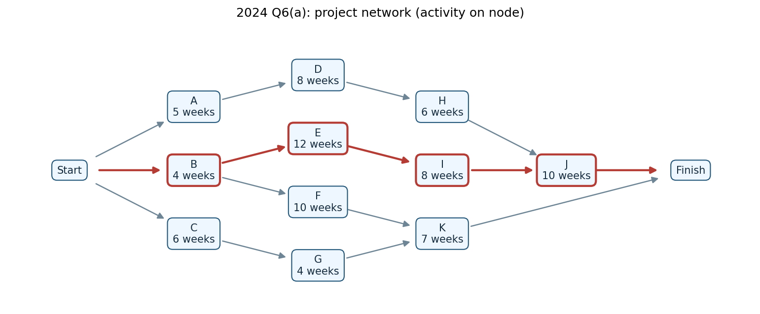
Activity A B C D E F G H I J K Preceding activity — — — A B B C D E H,I F,G Duration (weeks) 5 4 6 8 12 10 4 6 8 10 7 (i) Draw a network diagram of the project.
(ii) Determine the: I. critical path; II. project duration.
Model answer
| Activity | Predecessors | Duration | ES | EF | LS | LF | Float |
|---|---|---|---|---|---|---|---|
| A | — | 5 | 0 | 5 | 5 | 10 | 5 |
| B | — | 4 | 0 | 4 | 0 | 4 | 0 |
| C | — | 6 | 0 | 6 | 17 | 23 | 17 |
| D | A | 8 | 5 | 13 | 10 | 18 | 5 |
| E | B | 12 | 4 | 16 | 4 | 16 | 0 |
| F | B | 10 | 4 | 14 | 17 | 27 | 13 |
| G | C | 4 | 6 | 10 | 23 | 27 | 17 |
| H | D | 6 | 13 | 19 | 18 | 24 | 5 |
| I | E | 8 | 16 | 24 | 16 | 24 | 0 |
| J | H,I | 10 | 24 | 34 | 24 | 34 | 0 |
| K | F,G | 7 | 14 | 21 | 27 | 34 | 13 |
Forward pass: ES = latest predecessor EF; EF = ES + duration. Backward pass: LF = earliest successor LS; LS = LF − duration. Float = LS − ES. Project duration = 34 weeks. Red identifies critical activities and their controlling links.
Critical path: B → E → I → J. Duration = 4 + 12 + 8 + 10 = 34 weeks. Both terminal branches J and K must finish, so the later finish controls completion.
Question 6(b) — 8 marks
The following are the average prices of a certain commodity in a market.
Year Price Ksh 2013 15 2014 18 2015 20 2016 20 2017 19 2018 25 2019 26 2020 28 2021 28 2022 30 (i) Using the least squares method, determine the trend line equation.
(ii) Based on the equation in (i) above, estimate the price of the commodity in the year 2023.
Model answer
Centre time at 2017.5: x = year − 2017.5. Since Σx = 0, a = Σy/n and b = Σxy/Σx².
| Year | y | Centred x | x² | xy |
|---|---|---|---|---|
| 2013 | 15 | -4.50 | 20.25 | -67.50 |
| 2014 | 18 | -3.50 | 12.25 | -63 |
| 2015 | 20 | -2.50 | 6.25 | -50 |
| 2016 | 20 | -1.50 | 2.25 | -30 |
| 2017 | 19 | -0.50 | 0.25 | -9.50 |
| 2018 | 25 | 0.50 | 0.25 | 12.50 |
| 2019 | 26 | 1.50 | 2.25 | 39 |
| 2020 | 28 | 2.50 | 6.25 | 70 |
| 2021 | 28 | 3.50 | 12.25 | 98 |
| 2022 | 30 | 4.50 | 20.25 | 135 |
| Total | 229 | 0 | 82.50 | 134.50 |
| Step / item | Working | Result |
|---|---|---|
| Intercept a | 229/10 | 22.90 |
| Slope b | Σxy/Σx² | 1.63 |
| 2023 forecast | 22.900000 + 1.630303 × (2023 − 2017.5) | 31.87 |
Trend: ŷ = 22.9000 + 1.630303(year − 2017.5). Estimated 2023 price = Ksh 31.87.
Question 7(a) — 9 marks
The annual requirement of material TD at Ware Manufacturing Company is 1,200 units. The ordering cost is Ksh 2,500 per order, while the carrying cost is Ksh 600 per unit per year. Determine the:
(i) Economic Order Quantity (EOQ);
(ii) number of orders per year;
(iii) average inventory;
(iv) total relevant cost with the inventory.
Model answer
| Step / item | Working | Result |
|---|---|---|
| EOQ | √(2DS/H) = √(2×1,200×2,500/600) | 100 |
| Orders per year | 1,200/100 | 12 |
| Average inventory | 100/2 | 50 |
| Annual ordering cost | 12 × 2,500 | 30,000 |
| Annual holding cost | 50 × 600 | 30,000 |
| Total relevant annual cost | 30,000 + 30,000 | 60,000 |
This assumes steady demand, no shortages and no safety stock. Unit purchase price is not given and purchase expenditure is not relevant to the basic EOQ choice when unit price is constant.
Question 7(b) — 11 marks
Three assessors P, Q and R ranked 10 employees at Pendo Limited according to their accuracy in a certain task as follows:
Employee Assessor P Assessor Q Assessor R A 1 9 2 B 4 7 4 C 6 2 5 D 2 5 1 E 7 1 8 F 10 4 9 G 3 6 3 H 8 10 7 I 5 8 10 J 9 3 6 (i) Determine the Spearman’s Rank coefficient of correlation between: I. assessor P and assessor Q; II. assessor P and assessor R; III. assessor Q and assessor R.
(ii) Based on the results in (i) above, determine the pair of assessors whose judgement of accuracy were: I. most consistent; II. most inconsistent.
Model answer
No tied ranks occur. For each pair rₛ = 1 − 6Σd²/[n(n²−1)], with n = 10 and denominator 990.
| Employee | P | Q | R | (P−Q)² | (P−R)² | (Q−R)² |
|---|---|---|---|---|---|---|
| A | 1 | 9 | 2 | 64 | 1 | 49 |
| B | 4 | 7 | 4 | 9 | 0 | 9 |
| C | 6 | 2 | 5 | 16 | 1 | 9 |
| D | 2 | 5 | 1 | 9 | 1 | 16 |
| E | 7 | 1 | 8 | 36 | 1 | 49 |
| F | 10 | 4 | 9 | 36 | 1 | 25 |
| G | 3 | 6 | 3 | 9 | 0 | 9 |
| H | 8 | 10 | 7 | 4 | 1 | 9 |
| I | 5 | 8 | 10 | 9 | 25 | 4 |
| J | 9 | 3 | 6 | 36 | 9 | 9 |
| Total | 228 | 40 | 188 |
| Pair | Σd² | rₛ |
|---|---|---|
| P and Q | 228 | -0.381818 |
| P and R | 40 | 0.757576 |
| Q and R | 188 | -0.139394 |
P and R are most consistent because they have the highest positive correlation. P and Q are most inconsistent because they have the lowest (most negative) correlation.