Managerial Accounting — 2020
KNEC Diploma in Supply Chain Management, Module III. Original examination questions with explained answers for revision. Answers are independently prepared for study and are not an official KNEC marking scheme.
July 2020
Paper codes: 2903/305; 2906/305; 2907/305; 2926/305; 3103
Question 1(a) — 8 marks
Explain four production related decisions made in Managerial Accounting.
Answer
- Make or buy: compare avoidable internal production costs and capacity opportunity costs with the price of purchasing externally.
- Product mix: allocate scarce materials, machine time or labour to products with the best contribution per limiting resource.
- Continue or discontinue: assess the contribution lost and costs actually saved when a product or production line is closed.
- Capacity and production method: compare the relevant costs and benefits of machinery, overtime, subcontracting or process changes needed to meet output requirements.
Question 1(b) — 12 marks
Tamara Limited manufactures a single product, TM. The following is the extract of the budgeted income statement for the year 2021.
Item Ksh Sales (80,000 units) 8,000,000 Variable costs 3,200,000 Fixed costs 3,600,000 Total costs 6,800,000 Net profit 1,200,000 Determine the:
(i) break-even point in units and in shillings;
(ii) margin of safety in units and in percentage;
(iii) the number of units to be sold in order to make a profit of Ksh 3,300,000;
(iv) selling price required to make a profit of Ksh 3,600,000, based on the current sales of 80,000 units.
Answer
| Item | Working | Result |
|---|---|---|
| Selling price/unit | 8,000,000 ÷ 80,000 | 100 |
| Variable cost/unit | 3,200,000 ÷ 80,000 | 40 |
| Contribution/unit | 100 − 40 | 60 |
| Break-even units | 3,600,000 ÷ 60 | 60,000 |
| Break-even sales | 60,000 × 100 | 6,000,000 |
| MOS units | 80,000 − 60,000 | 20,000 |
| MOS percentage | 20,000 ÷ 80,000 × 100 | 25% |
| Units for Ksh 3.3m profit | (3,600,000 + 3,300,000) ÷ 60 | 115,000 |
| Price for Ksh 3.6m profit | (3,200,000 + 3,600,000 + 3,600,000) ÷ 80,000 | 130 |
Question 2(a) — 8 marks
Explain each of the following transfer pricing methods:
(i) Full cost transfer pricing.
(ii) Marginal cost transfer pricing.
(iii) Market based transfer pricing.
(iv) Negotiated transfer pricing.
Answer
- Full cost: charge the receiving division the production cost including allocated fixed overhead; a profit mark-up may be added if specified.
- Marginal cost: use the variable or incremental cost of supplying the transferred units; if capacity is constrained, the minimum acceptable price also includes contribution forgone.
- Market based: use a comparable external market price, adjusted for selling or distribution costs avoided on internal transfers.
- Negotiated: divisional managers agree a price within a range acceptable to both, subject to group objectives and capacity constraints.
Question 2(b) — 12 marks
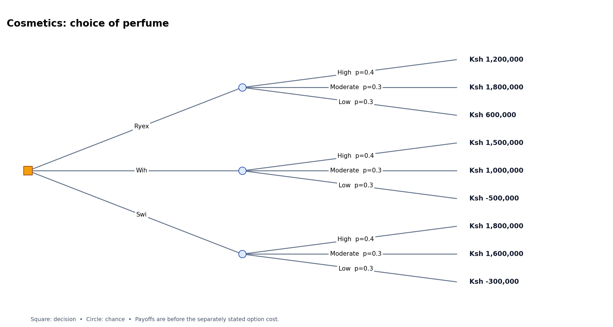
Cosmetics Limited intends to introduce a new perfume in the market. Three types of perfumes have been proposed by the management; Ryex, Wih and Swi. The following data relates to the expected demand, probabilities and expected annual net profits for the three perfumes:
Demand Probability Ryex (Ksh ‘000) Wih (Ksh ‘000) Swi (Ksh ‘000) High 0.40 1,200 1,500 1,800 Moderate 0.30 1,800 1,000 1,600 Low 0.30 600 -500 -300 (i) Draw a decision tree to represent the information above.
(ii) Determine the Expected Monetary Value (EMV) of each perfume.
(iii) Based on the results in (ii) above, advise the management on the perfume to introduce in the market.
Answer
- Introduce Ryex under the EMV criterion. Its expected annual net profit of Ksh. 1,200,000 exceeds Swi’s Ksh. 1,110,000 and Wih’s Ksh. 750,000. Keep the low-demand losses for Wih and Swi negative.
| Alternative | Σ probability × payoff | Expected gross payoff | Option cost | Net EMV (Ksh) |
|---|---|---|---|---|
| Ryex | 0.4 × (1,200,000) + 0.3 × (1,800,000) + 0.3 × (600,000) | 1,200,000 | 0 | 1,200,000 |
| Wih | 0.4 × (1,500,000) + 0.3 × (1,000,000) + 0.3 × (-500,000) | 750,000 | 0 | 750,000 |
| Swi | 0.4 × (1,800,000) + 0.3 × (1,600,000) + 0.3 × (-300,000) | 1,110,000 | 0 | 1,110,000 |
Question 3(a) — 8 marks
Malipi Transporters owns a fleet of vehicles for logistic purposes. The following data shows the number of years that the vehicles have been used and their respective maintenance costs:
Number of years used 2 4 6 10 12 15 Maintenance cost (Ksh ‘000) 2 3 3 5 8 10 (i) Determine the linear regression equation.
(ii) Using the equation in (i) above, estimate the maintenance cost of a vehicle that has been used for 18 years.
Answer
| Years used x | Maintenance cost y (Ksh ‘000) | x² | xy |
|---|---|---|---|
| 2 | 2 | 4 | 4 |
| 4 | 3 | 16 | 12 |
| 6 | 3 | 36 | 18 |
| 10 | 5 | 100 | 50 |
| 12 | 8 | 144 | 96 |
| 15 | 10 | 225 | 150 |
| Σ | 31 | 525 | 330 |
| Item | Working | Result |
|---|---|---|
| Totals | n=6; Σx=49; Σy=31 | |
| Slope b | [6 × 330 − 49 × 31] ÷ [6 × 525 − 49²] | 0.615487 |
| Intercept a | [31 − (0.615487 × 49)] ÷ 6 | 0.140187 |
| Regression equation | ŷ = a + bx | ŷ = 0.140187 + (0.615487)x |
| Prediction at x=18 | 0.140187 + (0.615487 × 18) | 11.22 |
The estimated maintenance cost is Ksh. 11,218.96. This is an extrapolation beyond the observed 2–15 years.
Question 3(b) — 12 marks
Naxim Limited intends to purchase either machine A or machine B. The cost of each machine is Ksh 1,000,000. The following are the expected net cash inflows from each of the machines.
Year Machine A (Ksh) Machine B (Ksh) 1 200,000 200,000 2 390,000 400,000 3 300,000 330,000 4 330,000 540,000 Additional information: The cost of capital is 14%. The scrap values at the end of the four years are Ksh 80,000 for A and Ksh 100,000 for B.
(i) For each of the projects, calculate the Net Present Value (NPV).
(ii) Based on the results in (i) above, advise the management on the machine to purchase.
Answer
- Add scrap proceeds to the final-year operating inflow only: A’s year-4 cash flow is Ksh. 410,000 and B’s is Ksh. 640,000.
- Purchase machine B. NPV B is Ksh. 84,897.59, compared with NPV A of Ksh. -79,224.70; B has the higher positive NPV.
Machine A, including scrap: discount rate 14%. PV = cash flow ÷ (1 + r)ⁿ. All amounts are Ksh.
| Year | Net cash flow | Discount factor | Present value |
|---|---|---|---|
| 1 | 200,000 | 0.877193 | 175,438.60 |
| 2 | 390,000 | 0.769468 | 300,092.34 |
| 3 | 300,000 | 0.674972 | 202,491.45 |
| 4 | 410,000 | 0.592080 | 242,752.91 |
| Total PV | 920,775.30 | ||
| Initial investment (time 0) | -1,000,000 | ||
| NPV | -79,224.70 |
Machine B, including scrap: discount rate 14%. PV = cash flow ÷ (1 + r)ⁿ. All amounts are Ksh.
| Year | Net cash flow | Discount factor | Present value |
|---|---|---|---|
| 1 | 200,000 | 0.877193 | 175,438.60 |
| 2 | 400,000 | 0.769468 | 307,787.01 |
| 3 | 330,000 | 0.674972 | 222,740.60 |
| 4 | 640,000 | 0.592080 | 378,931.38 |
| Total PV | 1,084,897.59 | ||
| Initial investment (time 0) | -1,000,000 | ||
| NPV | 84,897.59 |
Question 4(a) — 8 marks
Hitoch Computers Limited intends to hire 4 computer technicians; John, Jane, Joyce and Joseph. They are to offer computer maintenance services to their four clients; K, L, M and N. The amount chargeable, in thousands of shillings, by each of the computer technicians to each of the clients is as shown below:
Technician K L M N John 4 7 8 2 Jane 10 8 12 10 Joyce 5 8 10 14 Joseph 16 10 12 13 Determine the:
(i) assignment schedule that will minimize total cost;
(ii) minimum total cost.
Answer
Apply the Hungarian method. Reduce each row by its smallest entry, then reduce each column by its smallest entry.
After row reduction:
| K | L | M | N | |
|---|---|---|---|---|
| John | 2 | 5 | 6 | 0 |
| Jane | 2 | 0 | 4 | 2 |
| Joyce | 0 | 3 | 5 | 9 |
| Joseph | 6 | 0 | 2 | 3 |
After column reduction:
| K | L | M | N | |
|---|---|---|---|---|
| John | 2 | 5 | 4 | 0 |
| Jane | 2 | 0 | 2 | 2 |
| Joyce | 0 | 3 | 3 | 9 |
| Joseph | 6 | 0 | 0 | 3 |
Choose four independent zeros, with one assignment in every row and column. Read the values from the original table:
| Assign | To | Ksh ‘000 |
|---|---|---|
| John | N | 2 |
| Jane | L | 8 |
| Joyce | K | 5 |
| Joseph | M | 12 |
| Minimum | 27 |
Minimum total cost = Ksh. 27,000.
Question 4(b) — 12 marks
Alexip Company has three factories: A, B and C which supply refrigerators to four supermarkets: D, E, F and G, on a monthly basis. The monthly factory capacities are as shown below:
Factory Refrigerators available A 80 B 100 C 115 The monthly requirements for each supermarket are as follows:
Supermarket Refrigerators required D 50 E 60 F 80 G 105 The cost of transporting one unit, in Kenya shillings, from each factory to each supermarket is as follows:
Factory D E F G A 170 200 130 120 B 160 210 260 250 C 150 140 180 170 Using the least cost method, determine the:
(i) basic transportation schedule;
(ii) minimum cost of transportation.
Answer
Least cost allocation steps:
| Step | Route | Selection | Quantity |
|---|---|---|---|
| 1 | A → G | unit cost 120 | 80 |
| 2 | C → E | unit cost 140 | 60 |
| 3 | C → D | unit cost 150 | 50 |
| 4 | C → G | unit cost 170 | 5 |
| 5 | B → G | unit cost 250 | 20 |
| 6 | B → F | unit cost 260 | 80 |
Initial basic feasible schedule:
| Source → destination | D | E | F | G | Supply |
|---|---|---|---|---|---|
| A | 0 | 0 | 0 | 80 | 80 |
| B | 0 | 0 | 80 | 20 | 100 |
| C | 50 | 60 | 0 | 5 | 115 |
| Demand | 50 | 60 | 80 | 105 | 295 |
Initial transportation cost = Σ(quantity × unit cost) = 52,150 Ksh.
The initial allocation method produces a feasible schedule, but does not by itself prove minimum cost. Apply MODI: uᵢ + vⱼ = cᵢⱼ on basic cells and Δᵢⱼ = cᵢⱼ − uᵢ − vⱼ on nonbasic cells. A negative Δ permits a cost reduction; adjust alternating +/− cells by θ. Zero basic allocations may be used for degeneracy.
| Iteration | Entering route | Δ per unit | θ | Alternating loop | New total cost |
|---|---|---|---|---|---|
| 1 | B → D | -70 | 20 | +B→D; −C→D; +C→G; −B→G | 50,750 |
| 2 | A → F | -70 | 30 | +A→F; −B→F; +B→D; −C→D; +C→G; −A→G | 48,650 |
| 3 | B → E | -10 | 50 | +B→E; −C→E; +C→G; −A→G; +A→F; −B→F | 48,150 |
| 4 | C → F | -10 | 0 | +C→F; −B→F; +B→E; −C→E | 48,150 |
Optimal schedule:
| Source → destination | D | E | F | G | Supply |
|---|---|---|---|---|---|
| A | 0 | 0 | 80 | 0 | 80 |
| B | 50 | 50 | 0 | 0 | 100 |
| C | 0 | 10 | 0 | 105 | 115 |
| Demand | 50 | 60 | 80 | 105 | 295 |
| Row potentials u | A | B | C |
|---|---|---|---|
| Value | 0 | 120 | 50 |
| Column potentials v | D | E | F | G |
|---|---|---|---|---|
| Value | 40 | 90 | 130 | 120 |
Final reduced costs (all are nonnegative, proving optimality):
| D | E | F | G | |
|---|---|---|---|---|
| A | 130 | 110 | 0 | 0 |
| B | 0 | 0 | 10 | 10 |
| C | 60 | 0 | 0 | 0 |
Cost working: 80 × 130 + 50 × 160 + 50 × 210 + 10 × 140 + 105 × 170 = 48,150 Ksh.
Question 5(a) — 8 marks
Muliku Limited produces and sells 3 products: X, Y and Z. The following data relates to the products for the month of October 2019:
Item (Ksh) X Y Z Sales 300,000 230,000 200,000 Total costs 250,000 250,000 150,000 Net profit / loss 50,000 -20,000 50,000 The total costs comprise of 80% variable costs and 20% fixed costs. The management is contemplating dropping product Y. Advise the management on whether to drop product Y or not.
Answer
- Keep Y if its fixed costs remain. Y contributes Ksh. 30,000 towards fixed costs, despite an allocated loss of Ksh. 20,000. Dropping it reduces total profit from Ksh. 80,000 to Ksh. 50,000.
- A different conclusion would require avoidable fixed costs above the lost contribution, or a more profitable alternative use of capacity; neither is stated.
| Marginal statement (Ksh) | X | Y | Z | Total |
|---|---|---|---|---|
| Sales | 300,000 | 230,000 | 200,000 | 730,000 |
| Variable costs | 200,000 | 200,000 | 120,000 | 520,000 |
| Contribution | 100,000 | 30,000 | 80,000 | 210,000 |
| Fixed costs | 50,000 | 50,000 | 30,000 | 130,000 |
| Profit / loss | 50,000 | -20,000 | 50,000 | 80,000 |
Question 5(b) — 12 marks
Napon Limited manufactures and sells a single product, Km. The following costs relate to the production of 10,000 units of the product for the year 2018:
Cost Ksh Raw materials 2,000,000 Managers salaries 2,500,000 Factory rent 1,000,000 Administration cost (60% variable) 1,500,000 Direct labour 1,000,000 Electricity (40% fixed) 600,000 (i) Using the accounts analysis method, determine: I total fixed costs; II variable cost per unit. (ii) Based on the results in (i), formulate the linear cost function in the form y = a + bx. (iii) Determine the increase in total cost when 12,000 units are produced in a year.
Answer
| Cost (Ksh) | Total | Fixed portion | Variable portion |
|---|---|---|---|
| Raw materials | 2,000,000 | 0 | 2,000,000 |
| Managers salaries | 2,500,000 | 2,500,000 | 0 |
| Factory rent | 1,000,000 | 1,000,000 | 0 |
| Administration | 1,500,000 | 600,000 | 900,000 |
| Direct labour | 1,000,000 | 0 | 1,000,000 |
| Electricity | 600,000 | 240,000 | 360,000 |
| Total | 8,600,000 | 4,340,000 | 4,260,000 |
| Item | Working | Result |
|---|---|---|
| Variable cost per unit | 4,260,000 ÷ 10,000 | 426 |
| Total fixed cost | Sum of fixed portions | 4,340,000 |
| Linear cost function | Y = a + bx | Y = 4,340,000 + 426x |
| Cost at 12,000 units | 4,340,000 + 426 × 12,000 | 9,452,000 |
| Item | Working | Result |
|---|---|---|
| Current total cost at 10,000 units | 4,340,000 + 426 × 10,000 | 8,600,000 |
| Increase in total cost | 426 × (12,000 − 10,000) | 852,000 |
Question 6(a) — 8 marks
Highlight four limitations of the cost-volume-profit (CVP) analysis.
Answer
- Constant selling price is assumed, although discounts and market changes may alter revenue per unit.
- Costs are treated as linear, with constant variable cost per unit and fixed costs within a relevant range; overtime or capacity steps can break this assumption.
- Costs must be separated reliably into fixed and variable elements, which is difficult for mixed costs.
- A single product or constant sales mix is assumed; changes in the mix alter the average contribution and break-even point.
Question 6(b) — 12 marks
Bingwa Limited manufactures and sells two types of products Jx and Kx, using two types of materials; M1 and M2.
The following are the estimates for the month of January 2022:
Expected sales Units Selling price/unit (Ksh) Jx 600 200 Kx 400 250
Standard material kg/unit Jx Kx M1 4 1 M2 2 2
Material Cost/kg (Ksh) M1 100 M2 150
Finished goods inventory Jx Kx 1 January 50 80 31 January 40 50
Raw materials inventory (kg) M1 M2 1 January 40 50 31 January 60 70 For the month of January 2022, prepare:
(i) sales budget in shillings;
(ii) production budget in units;
(iii) material usage budget in units;
(iv) material purchases budget in shillings.
Answer
Sales budget:
| Product | Sales units | Price (Ksh) | Sales value (Ksh) |
|---|---|---|---|
| Jx | 600 | 200 | 120,000 |
| Kx | 400 | 250 | 100,000 |
| Total | 220,000 |
Production = sales + closing finished goods − opening finished goods:
| Product | Sales | Add closing | Less opening | Produce units |
|---|---|---|---|---|
| Jx | 600 | 40 | 50 | 590 |
| Kx | 400 | 50 | 80 | 370 |
Material usage budget (kg):
| Material | Jx | Kx | Total kg |
|---|---|---|---|
| M1 | 2,360 | 370 | 2,730 |
| M2 | 1,180 | 740 | 1,920 |
Purchases = usage + closing raw material − opening raw material:
| Material | Usage kg | Add closing kg | Less opening kg | Purchase kg | Cost/kg (Ksh) | Purchases (Ksh) |
|---|---|---|---|---|---|---|
| M1 | 2,730 | 60 | 40 | 2,750 | 100 | 275,000 |
| M2 | 1,920 | 70 | 50 | 1,940 | 150 | 291,000 |
| Total | 566,000 |
Question 7(a) — 8 marks
The management of Adepa Petrol station has ascertained that the arrivals and services at their facility follow a Poisson distribution. The average time between arrival of cars is 5 minutes while the average time taken to fuel a car is 2.5 minutes.
I. Determine: (i) expected average queue length; (ii) average number of cars in the queuing system. II. Mary is late for a meeting and has no time to wait in the queue. Determine the probability that the station will be busy on her arrival.
Answer
- For a Poisson arrival process, an arriving customer sees the long-run busy proportion. Therefore the probability that Mary finds the station busy is ρ = 0.5, or 50%.
λ = 60/5 = 12 cars per hour; μ = 60/2.5 = 24 cars per hour.
Use the stable M/M/1 model: one server, Poisson arrivals, independent exponential service times and λ < μ. Service completions are counted per time interval; service durations are exponential.
| Item | Working | Result |
|---|---|---|
| Arrival rate λ | Convert arrivals to an hourly rate | 12 per hour |
| Service rate μ | Convert services to an hourly rate | 24 per hour |
| Busy proportion ρ | λ / μ | 0.5000 = 50.00% |
| Idle proportion P₀ | 1 − ρ | 0.5000 = 50.00% |
| Mean queue length Lq | λ² / [μ(μ − λ)] | 0.50 |
| Mean number in system L | λ / (μ − λ) | 1 |
| Mean time in system W | 1 / (μ − λ) | 0.083333 hour = 5 minutes |
| Mean waiting time Wq | λ / [μ(μ − λ)] | 0.041667 hour = 2.5 minutes = 150 seconds |
Question 7(b) — 12 marks
Sandimix Limited has four storage sites for construction sand: S1, S2, S3 and S4. Four clients, C1, C2, C3 and C4 require to be supplied with sand. The quantities of sand available from each site is shown below:
Site Tonnes available S1 800 S2 700 S3 500 S4 600 The quantities required by each client are as shown below:
Client Tonnes required C1 500 C2 1,000 C3 700 C4 400 The cost of transporting one tonne of sand, in thousands of Kenya shillings, from each site to each client, is as shown below:
Site C1 C2 C3 C4 S1 2 4 6 8 S2 4 6 7 5 S3 9 3 6 7 S4 6 8 4 6 Using the Vogel’s approximation method (VAM), determine the:
(i) basic transportation schedule;
(ii) minimum cost of transportation.
Answer
VAM allocation steps:
| Step | Route | Selection | Quantity |
|---|---|---|---|
| 1 | S3 → C2 | row S3; penalty 3 | 500 |
| 2 | S1 → C1 | row S1; penalty 2 | 500 |
| 3 | S4 → C3 | row S4; penalty 2 | 600 |
| 4 | S2 → C4 | column C4; penalty 3 | 400 |
| 5 | S1 → C2 | row S1; penalty 2 | 300 |
| 6 | S2 → C3 | column C3; penalty 7 | 100 |
| 7 | S2 → C2 | row S2; penalty 6 | 200 |
Initial basic feasible schedule:
| Source → destination | C1 | C2 | C3 | C4 | Supply |
|---|---|---|---|---|---|
| S1 | 500 | 300 | 0 | 0 | 800 |
| S2 | 0 | 200 | 100 | 400 | 700 |
| S3 | 0 | 500 | 0 | 0 | 500 |
| S4 | 0 | 0 | 600 | 0 | 600 |
| Demand | 500 | 1,000 | 700 | 400 | 2,600 |
Initial transportation cost = Σ(quantity × unit cost) = 10,000 Ksh ‘000.
The initial allocation method produces a feasible schedule, but does not by itself prove minimum cost. Apply MODI: uᵢ + vⱼ = cᵢⱼ on basic cells and Δᵢⱼ = cᵢⱼ − uᵢ − vⱼ on nonbasic cells. A negative Δ permits a cost reduction; adjust alternating +/− cells by θ. Zero basic allocations may be used for degeneracy.
No improving negative reduced cost exists in the initial schedule.
Optimal schedule:
| Source → destination | C1 | C2 | C3 | C4 | Supply |
|---|---|---|---|---|---|
| S1 | 500 | 300 | 0 | 0 | 800 |
| S2 | 0 | 200 | 100 | 400 | 700 |
| S3 | 0 | 500 | 0 | 0 | 500 |
| S4 | 0 | 0 | 600 | 0 | 600 |
| Demand | 500 | 1,000 | 700 | 400 | 2,600 |
| Row potentials u | S1 | S2 | S3 | S4 |
|---|---|---|---|---|
| Value | 0 | 2 | -1 | -1 |
| Column potentials v | C1 | C2 | C3 | C4 |
|---|---|---|---|---|
| Value | 2 | 4 | 5 | 3 |
Final reduced costs (all are nonnegative, proving optimality):
| C1 | C2 | C3 | C4 | |
|---|---|---|---|---|
| S1 | 0 | 0 | 1 | 5 |
| S2 | 0 | 0 | 0 | 0 |
| S3 | 8 | 0 | 2 | 5 |
| S4 | 5 | 5 | 0 | 4 |
Cost working: 500 × 2 + 300 × 4 + 200 × 6 + 100 × 7 + 400 × 5 + 500 × 3 + 600 × 4 = 10,000 Ksh ‘000.
The minimum total cost in shillings is Ksh. 10,000,000.