Managerial Accounting — 2019
KNEC Diploma in Supply Chain Management, Module III. Original examination questions with explained answers for revision. Answers are independently prepared for study and are not an official KNEC marking scheme.
November 2019
Paper codes: 2903/305; 2906/305; 2907/305; 2926/305; 3103
Question 1(a) — 8 marks
John has been appointed as a Management Accountant at Wedy Enterprises. Explain four types of duties that he will perform in such a capacity.
Answer
- Planning: prepare forecasts, budgets and cost estimates that turn objectives into measurable resource requirements.
- Decision support: compare relevant future revenues and costs of alternatives such as making or buying, pricing and investing.
- Control: compare actual results with budgets, investigate significant variances and recommend corrective action.
- Performance evaluation: report controllable results for responsibility centres so managers can assess efficiency and achievement of targets.
Question 1(b) — 12 marks
Companies A and B sell the same type of product in the market. The following are the expected profit and loss accounts for the year ending 31 December 2018:
Item (Ksh) Company A Company B Sales 300,000 300,000 Variable costs 240,000 200,000 Fixed cost 30,000 70,000 Total costs 270,000 270,000 Profit 30,000 30,000 (i) For each company, calculate: (I) profit-volume (P/V) ratio; (II) break-even point (BEP) in shillings. (ii) Based on the results in (i), advise an investor which company to invest in to earn greater profit under conditions of: (I) high demand for the product; (II) low demand for the product.
Answer
- A’s P/V ratio is 20%; B’s is 33⅓%. A breaks even at Ksh. 150,000 sales and B at Ksh. 210,000.
- For high demand above the common Ksh. 300,000 sales point, choose B because its higher contribution ratio produces more additional profit for each shilling of sales.
- For low demand below that sales point, choose A because its lower fixed costs reduce losses and its break-even point is lower. At sales of Ksh. 300,000, both make Ksh. 30,000.
| Working | A | B |
|---|---|---|
| Contribution | 300,000 − 240,000 = 60,000 | 300,000 − 200,000 = 100,000 |
| P/V ratio | 60,000 / 300,000 = 20% | 100,000 / 300,000 = 33⅓% |
| Break-even sales | 30,000 / .20 = 150,000 | 70,000 / (1/3) = 210,000 |
| Profit at sales S | .20S − 30,000 | (1/3)S − 70,000 |
| Item | Working | Result |
|---|---|---|
| Equal-profit sales | (70,000 − 30,000) ÷ (1/3 − .20) | 300,000 |
Question 2(a) — 10 marks
The following data has been extracted from the books of account of Urembu Limited:
Sales volume x (printed Ksh) Amount of bad debts y (Ksh) 4,000 22,000 26,000 80,000 34,000 112,000 14,000 66,000 2,000 16,000 18,000 70,000 (i) Using the method of least squares, determine the regression equation of amount of bad debts on sales volume.
(ii) Based on the equation in (i) above, estimate the amount of bad debts when the sales volume is 20,000 units.
Answer
The table labels sales volume in Ksh, while the final requirement calls it units. Use the numerical x scale supplied; clarify its economic unit before applying the equation to a real business forecast.
| Sales volume x | Bad debts y (Ksh) | x² | xy |
|---|---|---|---|
| 4,000 | 22,000 | 16,000,000 | 88,000,000 |
| 26,000 | 80,000 | 676,000,000 | 2,080,000,000 |
| 34,000 | 112,000 | 1,156,000,000 | 3,808,000,000 |
| 14,000 | 66,000 | 196,000,000 | 924,000,000 |
| 2,000 | 16,000 | 4,000,000 | 32,000,000 |
| 18,000 | 70,000 | 324,000,000 | 1,260,000,000 |
| Σ | 366,000 | 2,372,000,000 | 8,192,000,000 |
| Item | Working | Result |
|---|---|---|
| Totals | n=6; Σx=98,000; Σy=366,000 | |
| Slope b | [6 × 8,192,000,000 − 98,000 × 366,000] ÷ [6 × 2,372,000,000 − 98,000²] | 2.870354 |
| Intercept a | [366,000 − (2.870354 × 98,000)] ÷ 6 | 14117.545376 |
| Regression equation | ŷ = a + bx | ŷ = 14117.545376 + (2.870354)x |
| Prediction at x=20000 | 14117.545376 + (2.870354 × 20000) | 71,524.63 |
Question 2(b) — 10 marks
The customers’ arrival at a barbershop manned by one barber follows a Poisson distribution, at an average rate of 3 customers per hour. Service at the barbershop is distributed exponentially, at an average rate of 5 customers per hour. Determine the:
(i) average number of customers waiting to be served;
(ii) average number of customers in the barbershop;
(iii) average time a customer waits until it reaches his turn;
(iv) average time a customer spends in the barbershop;
(v) percentage of time that the barber is busy.
Answer
Use the stable M/M/1 model: one server, Poisson arrivals, independent exponential service times and λ < μ. Service completions are counted per time interval; service durations are exponential.
| Item | Working | Result |
|---|---|---|
| Arrival rate λ | Convert arrivals to an hourly rate | 3 per hour |
| Service rate μ | Convert services to an hourly rate | 5 per hour |
| Busy proportion ρ | λ / μ | 0.6000 = 60.00% |
| Idle proportion P₀ | 1 − ρ | 0.4000 = 40.00% |
| Mean queue length Lq | λ² / [μ(μ − λ)] | 0.90 |
| Mean number in system L | λ / (μ − λ) | 1.50 |
| Mean time in system W | 1 / (μ − λ) | 0.500000 hour = 30 minutes |
| Mean waiting time Wq | λ / [μ(μ − λ)] | 0.300000 hour = 18 minutes = 1080 seconds |
Question 3(a) — 10 marks
Explain five advantages of the Net Present Value (NPV) method of investment appraisal.
Answer
- Time value of money: discounting recognises that a shilling received sooner is worth more than one received later.
- Whole-life cash flows: include relevant inflows and outflows throughout the project, including terminal proceeds, rather than stopping at payback.
- Direct value measure: a positive NPV measures the expected addition to value after recovering the investment and required return.
- Cash-flow basis: use relevant cash movements rather than accounting profits distorted by noncash depreciation or allocation methods.
- Consistent comparison and additivity: discount at an appropriate required return; NPVs of independent projects can be added when evaluating a portfolio, with due regard to resource constraints.
Question 3(b) — 10 marks
The following information relates to Maweto Limited:
2017 actual Ksh Sales (80,000 units) 200,000 Raw materials 106,000 Labour 22,000 Variable overhead 32,000 Fixed overhead 20,000 2018 estimates: Sales (120,000 units) Ksh 300,000. Raw materials: 5% increase in price. Labour: 15% increase in wage rate; 10% increase in productivity. New machines: Machine A Ksh 50,000; Machine B Ksh 24,000. 15% depreciation on cost to be provided. Prepare a budgeted income statement for the year 2018.
Answer
- Output rises from 80,000 to 120,000 units, a factor of 1.5. A 10% productivity improvement means labour hours per unit are divided by 1.10, not reduced by an arbitrary 10% of total wages.
- The Ksh. 74,000 machine purchases are capital expenditure. Charge the stated annual depreciation of Ksh. 11,100 to this income statement; do not also expense their full purchase cost. Assume existing fixed overhead continues.
| Budgeted income statement 2018 (Ksh) | Working | Amount |
|---|---|---|
| Sales | Given | 300,000 |
| Raw materials | 106,000 × 1.5 × 1.05 | 166,950 |
| Labour | 22,000 × 1.5 × 1.15 ÷ 1.10 | 34,500 |
| Variable overhead | 32,000 × 1.5 | 48,000 |
| Existing fixed overhead | Unchanged | 20,000 |
| New machine depreciation | (50,000 + 24,000) × 15% | 11,100 |
| Total costs | 280,550 | |
| Budgeted profit | 300,000 − 280,550 | 19,450 |
Question 4(a) — 8 marks
Explain each of the following terms as used in queuing theory:
(i) Jockeying;
(ii) Balking;
(iii) Reneging;
(iv) Collusion.
Answer
- Jockeying: moving from one waiting line to another in the hope of receiving service sooner.
- Balking: deciding not to join a queue after seeing its length or expected delay.
- Reneging: joining a queue, then leaving before receiving service because the wait becomes unacceptable.
- Collusion: customers cooperate to reduce or avoid separate waits, for example one customer combines requests for others. This can change the effective arrival or service pattern.
Question 4(b) — 12 marks
Pareto Limited intends to manufacture either product P or product Q. The following information relates to the two products.
Item P Q Selling price/unit (Ksh) 40 50 Variable manufacturing cost/unit (Ksh) 16 20 Fixed manufacturing cost (Ksh) 40,000 60,000 Fixed selling and administrative cost (Ksh) 20,000 30,000 Variable selling/admin cost per unit (Ksh) 8 10 Units produced 40,000 70,000 Units sold 38,000 65,000 (i) Using marginal costing approach, determine the profit of each product.
(ii) Based on the results in (i) above, advise the management on the product to manufacture.
Answer
- Use variable manufacturing cost to value closing inventory, and expense fixed manufacturing and fixed selling costs in the period. No opening inventory is supplied.
- Manufacture Q under the stated output and sales plan: it produces Ksh. 1,210,000 profit, compared with Ksh. 548,000 for P. If a scarce resource limits output, contribution per limiting resource would also need evaluation.
| Marginal income statement (Ksh) | P | Q |
|---|---|---|
| Sales | 1,520,000 | 3,250,000 |
| Variable manufacturing production | 640,000 | 1,400,000 |
| Less closing stock (2,000 × 16; 5,000 × 20) | -32,000 | -100,000 |
| Variable manufacturing cost of sales | 608,000 | 1,300,000 |
| Variable selling/admin (units sold × unit cost) | 304,000 | 650,000 |
| Contribution | 608,000 | 1,300,000 |
| Fixed manufacturing | 40,000 | 60,000 |
| Fixed selling/admin | 20,000 | 30,000 |
| Profit | 548,000 | 1,210,000 |
Question 5(a) — 8 marks
Mawingu Limited intends to invest Ksh 1,500,000 in a manufacturing plant. The following are the expected cash inflows from the manufacturing plant.
Year Cash inflow (Ksh) 1 600,000 2 400,000 3 200,000 4 100,000 5 800,000 The company’s cost of capital is 2%.
(i) Calculate the Net Present Value (NPV) of the plant.
(ii) Based on the results in (i) above, advise the management on whether to invest in the plant or not.
Answer
The supplied scan clearly prints 2%, so this answer uses 2% rather than substituting a more usual discount rate.
- Invest in the plant on the NPV criterion: NPV is positive at Ksh. 478,136.46 using the printed 2% cost of capital.
Mawingu plant: discount rate 2%. PV = cash flow ÷ (1 + r)ⁿ. All amounts are Ksh.
| Year | Net cash flow | Discount factor | Present value |
|---|---|---|---|
| 1 | 600,000 | 0.980392 | 588,235.29 |
| 2 | 400,000 | 0.961169 | 384,467.51 |
| 3 | 200,000 | 0.942322 | 188,464.47 |
| 4 | 100,000 | 0.923845 | 92,384.54 |
| 5 | 800,000 | 0.905731 | 724,584.65 |
| Total PV | 1,978,136.46 | ||
| Initial investment (time 0) | -1,500,000 | ||
| NPV | 478,136.46 |
Question 5(b) — 12 marks
Kwetu Limited is a manufacturing company that has four departments, A, B, C and D. The following information relates to the four departments for the year ended 31 December 2017:
Item (Ksh million) A B C D Total assets 36 30 42 54 Total annual sales 60 90 108 84 Total annual costs 54 81 96 78 (i) For each department, calculate the annual Return on Investment (ROI).
(ii) Based on the results in (i) above, rank the four departments according to their performance.
Answer
- Use total assets as the investment base because no separate opening or average investment figures are given. ROI = annual profit ÷ investment × 100.
- Performance ranking is B, C, A, D, from highest to lowest ROI. This relative percentage ranking does not by itself measure differences in business risk or absolute value created.
| Department | Profit (Ksh million) | ROI working | ROI | Rank |
|---|---|---|---|---|
| A | 60 − 54 = 6 | 6 ÷ 36 × 100 | 16.67% | 3 |
| B | 90 − 81 = 9 | 9 ÷ 30 × 100 | 30% | 1 |
| C | 108 − 96 = 12 | 12 ÷ 42 × 100 | 28.57% | 2 |
| D | 84 − 78 = 6 | 6 ÷ 54 × 100 | 11.11% | 4 |
Question 6(a) — 8 marks
Explain four disadvantages of decentralization in performance evaluation.
Answer
- Suboptimal decisions: a divisional manager may improve a local measure while harming total company profit, for example by refusing a beneficial internal transfer.
- Unfair comparisons: divisions facing different markets, asset ages or risk levels may be ranked misleadingly using the same unadjusted target.
- Measurement and allocation disputes: shared overheads, transfer prices and uncontrollable costs can distort reported divisional results.
- Duplication and coordination costs: separate reporting systems and management teams can increase costs and make consistent control more difficult.
Question 6(b) — 12 marks
A manufacturing company has three plants, A, B and C and three warehouses 1, 2 and 3. The following is the capacity of each plant, demand at each warehouse and the unit cost of transportation in thousands of shillings:
Plant 1 2 3 Capacity A 16 18 20 42 B 18 22 22 30 C 20 24 18 28 Demand 35 40 30 (i) Using the least cost method, determine the basic transportation schedule.
(ii) Based on the results in (i) above, determine the expected total cost of transportation.
Answer
- Total demand is 105 and capacity is 100, so no real shipment schedule can meet all stated demand. The dummy source balances the arithmetic while explicitly identifying 5 units of unmet demand.
- The requirement asks for a basic least-cost schedule and its expected cost. Ties can produce another feasible basic schedule; the schedule below follows the displayed allocation steps.
Demand exceeds available supply by 5. Add a dummy source of 5 at zero accounting transport cost to balance the tableau. Dummy allocations represent unmet demand, not actual deliveries; real shortage penalties are not supplied.
Least cost allocation steps:
| Step | Route | Selection | Quantity |
|---|---|---|---|
| 1 | Dummy (unmet demand) → 1 | unit cost 0 | 5 |
| 2 | A → 1 | unit cost 16 | 30 |
| 3 | C → 3 | unit cost 18 | 28 |
| 4 | A → 2 | unit cost 18 | 12 |
| 5 | B → 2 | unit cost 22 | 28 |
| 6 | B → 3 | unit cost 22 | 2 |
Initial basic feasible schedule:
| Source → destination | 1 | 2 | 3 | Supply |
|---|---|---|---|---|
| A | 30 | 12 | 0 | 42 |
| B | 0 | 28 | 2 | 30 |
| C | 0 | 0 | 28 | 28 |
| Dummy (unmet demand) | 5 | 0 | 0 | 5 |
| Demand | 35 | 40 | 30 | 105 |
Initial transportation cost = Σ(quantity × unit cost) = 1,860 Ksh ‘000.
The stated basic schedule costs Ksh. 1,860,000. No real shortage cost is provided.
Question 7(a) — 8 marks
A marketing manager would like to assign four salesmen 1, 2, 3 and 4 to four cities P, Q, R and S. The following is the profit to be realised by each salesman in each city, in thousands of shillings:
Salesman P Q R S 1 50 54 56 76 2 56 60 58 80 3 70 48 64 66 4 48 64 50 56 Determine the:
(i) salesman to be assigned to each city so as to maximise profits;
(ii) total maximum profit, related to the assignment in (i) above.
Answer
Maximise by converting each entry to an opportunity loss: 80 minus the original entry. Apply the Hungarian method. Reduce each row by its smallest entry, then reduce each column by its smallest entry.
After row reduction:
| P | Q | R | S | |
|---|---|---|---|---|
| 1 | 26 | 22 | 20 | 0 |
| 2 | 24 | 20 | 22 | 0 |
| 3 | 0 | 22 | 6 | 4 |
| 4 | 16 | 0 | 14 | 8 |
After column reduction:
| P | Q | R | S | |
|---|---|---|---|---|
| 1 | 26 | 22 | 14 | 0 |
| 2 | 24 | 20 | 16 | 0 |
| 3 | 0 | 22 | 0 | 4 |
| 4 | 16 | 0 | 8 | 8 |
Cover zeros with rows 3 and columns Q, S. Minimum uncovered entry = 8. Subtract it from uncovered cells and add it at line intersections.
| P | Q | R | S | |
|---|---|---|---|---|
| 1 | 18 | 22 | 6 | 0 |
| 2 | 16 | 20 | 8 | 0 |
| 3 | 0 | 30 | 0 | 12 |
| 4 | 8 | 0 | 0 | 8 |
Cover zeros with rows 3, 4 and columns S. Minimum uncovered entry = 6. Subtract it from uncovered cells and add it at line intersections.
| P | Q | R | S | |
|---|---|---|---|---|
| 1 | 12 | 16 | 0 | 0 |
| 2 | 10 | 14 | 2 | 0 |
| 3 | 0 | 30 | 0 | 18 |
| 4 | 8 | 0 | 0 | 14 |
Choose four independent zeros, with one assignment in every row and column. Read the values from the original table:
| Assign | To | Ksh ‘000 |
|---|---|---|
| 1 | R | 56 |
| 2 | S | 80 |
| 3 | P | 70 |
| 4 | Q | 64 |
| Maximum | 270 |
Maximum profit = Ksh. 270,000.
Question 7(b) — 12 marks
A company is planning on whether to develop and launch a new product or not. Research and development costs are expected to be Ksh. 1,300,000. There is a 75% chance that the product launch will be successful. If the launch is successful, the levels of expected profits may be high, medium or low. The following are the probabilities for each level of expected profits:
Success profit level Probability Profits (Ksh) High 0.30 2,000,000 Medium 0.60 1,600,000 Low 0.20 1,200,000 In the event that the launch is a failure, there is a probability of 0.7 that the research and development work can be sold for Ksh 100,000 and a probability of 0.3 that it will be worthless.
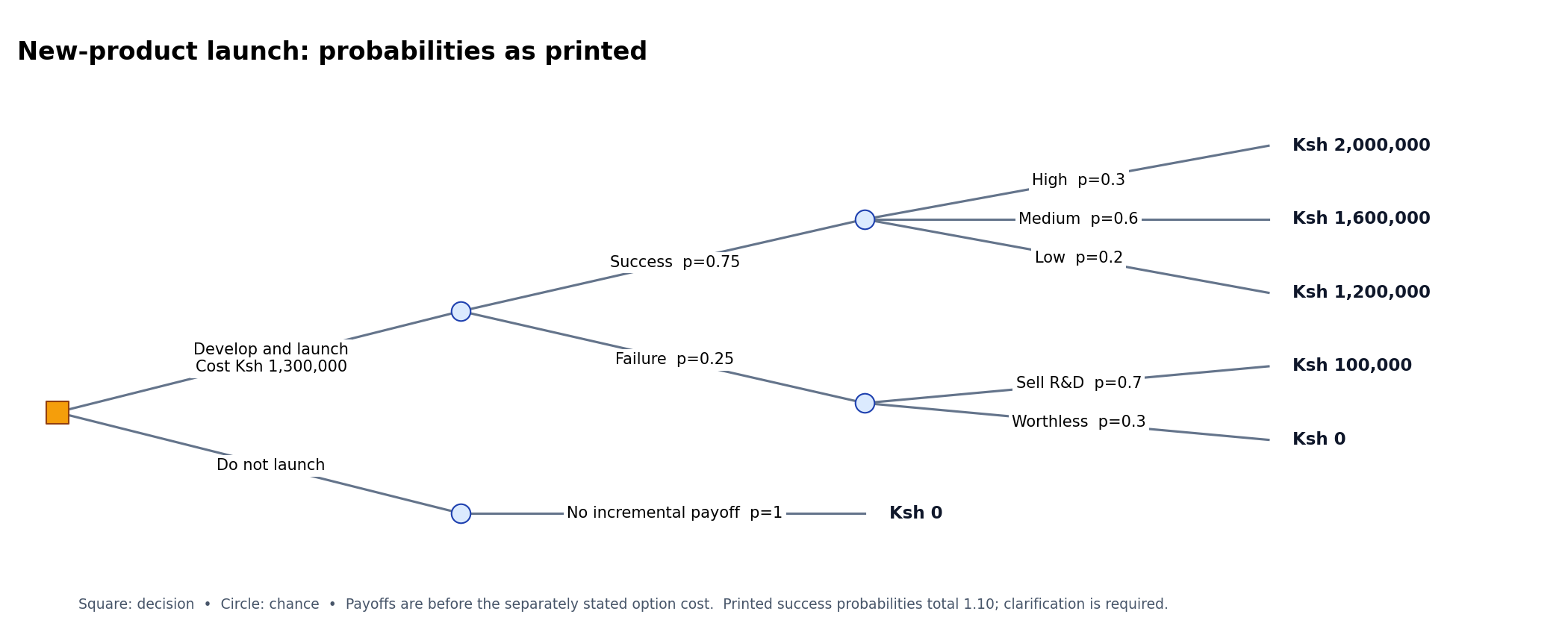
(i) Present the above information in a decision tree.
(ii) Based on the Expected Monetary Value (EMV) approach, advise the management on whether to develop and launch the new product or not.
Answer
- The success-state probabilities add to 1.10, so the printed information does not define a valid probability distribution. A unique valid EMV and an unconditional recommendation cannot be obtained without clarification.
- The tree preserves the source figures. As an explicitly illustrative assumption, normalise those three weights proportionally by dividing each by 1.10; do not present this assumption as a correction confirmed by the examiner.
- Under that assumption, net EMV is negative Ksh. 55,227.27, so do not launch. If a different printed probability is the error, the result changes; the actual decision requires corrected probabilities.
| Item | Working | Result |
|---|---|---|
| Probability check | .3 + .6 + .2 | 1.10 (invalid for mutually exclusive, exhaustive states) |
| Illustrative proportional normalisation | Divide each success-state weight by 1.10 | High .272727; medium .545455; low .181818 |
| Conditional success payoff | (.3 × 2,000,000 + .6 × 1,600,000 + .2 × 1,200,000) ÷ 1.10 | 1,636,363.64 |
| Conditional failure payoff | .7 × 100,000 + .3 × 0 | 70,000 |
| Illustrative net EMV | .75 × (1,800,000 ÷ 1.10) + .25 × 70,000 − 1,300,000 | -55,227.27 |